

Transform your Raspberry Pi into an intelligent decision-making system with Q-learning, a powerful reinforcement learning algorithm that excels at learning optimal actions through trial and error. By implementing Q-learning in Python, you can create sophisticated machine learning projects on Raspberry Pi that adapt and improve over time – from autonomous robots to smart home controllers.
Q-learning stands out for its ability to learn without a predefined model, making it ideal for real-world applications where perfect information isn’t available. The algorithm maintains a Q-table that maps state-action pairs to expected rewards, continuously updating these values as the agent interacts with its environment.
Python’s simple syntax and robust libraries like NumPy make implementing Q-learning straightforward, while the Raspberry Pi’s GPIO capabilities enable direct interaction with sensors and actuators. This combination creates a perfect platform for experimenting with reinforcement learning in physical computing projects.
Whether you’re building a self-balancing robot or creating an adaptive temperature control system, Q-learning provides the intelligence needed to make your projects truly autonomous. Let’s dive into the practical implementation and discover how this powerful algorithm can enhance your next Raspberry Pi project.
Setting Up Your Raspberry Pi for Q-Learning
Required Hardware Components
While Q-learning implementation in Python primarily relies on software, having the right hardware setup ensures smooth execution of your reinforcement learning projects. For basic Q-learning experiments, a standard computer with at least 8GB RAM and a modern multi-core processor will suffice. However, if you’re planning to work with more complex environments or larger datasets, consider exploring specialized hardware components for AI projects.
Essential components:
– Computer/laptop with Python environment
– Minimum 8GB RAM (16GB recommended)
– Multi-core processor (Intel i5/AMD Ryzen 5 or better)
– 20GB free storage space
Optional but recommended:
– GPU for faster training (NVIDIA GTX 1660 or better)
– External cooling system for extended training sessions
– Additional storage for saving model states
– Secondary display for monitoring training progress
For those using Raspberry Pi, ensure you have at least a Raspberry Pi 4 with 4GB RAM. While not optimal for complex Q-learning tasks, it’s perfect for learning and simple implementations. Remember to maintain proper cooling, as training sessions can be resource-intensive.
Software Installation and Dependencies
Before implementing Q-learning in Python, let’s set up our development environment with all the necessary dependencies. First, ensure you have Python 3.7 or later installed on your system. You can verify this by opening a terminal and running `python –version`.
To install the required libraries, open your terminal and use pip, Python’s package installer:
“`bash
pip install numpy
pip install gym
pip install matplotlib
“`
NumPy will handle our matrix operations, OpenAI Gym provides the environment for our Q-learning experiments, and Matplotlib helps us visualize the results.
For those using virtual environments (recommended), create and activate one first:
“`bash
python -m venv qlearning_env
source qlearning_env/bin/activate # On Windows, use: qlearning_env\Scripts\activate
“`
If you’re working with Jupyter notebooks, install and launch Jupyter:
“`bash
pip install jupyter
jupyter notebook
“`
These installations provide everything needed to start implementing Q-learning algorithms. Make sure all packages install successfully before proceeding with the implementation.
Understanding Q-Learning Fundamentals
Q-Learning Theory Made Simple
Think of Q-learning as teaching a robot to find the best route through a maze using trial and error, much like how we learn to play a new video game. The “Q” in Q-learning stands for “Quality” – essentially how good a particular action is in a given situation.
Imagine you’re teaching a dog new tricks. Initially, the dog tries random actions, but with treats (rewards), it learns which actions lead to the best outcomes. Q-learning works similarly: the algorithm learns by receiving rewards for its actions and updates its knowledge (stored in what we call a Q-table) accordingly.
Let’s use a simple real-world example: a robot learning to navigate a room to find a charging station. At first, the robot doesn’t know which direction to move. Through exploration, it discovers that moving toward the charging station yields positive rewards, while bumping into walls results in negative rewards. The robot gradually builds a Q-table that maps each position (state) and possible movement (action) to an expected reward value.
The beauty of Q-learning lies in its balance between exploration (trying new paths) and exploitation (using known successful paths). This balance ensures the algorithm doesn’t get stuck using only the first solution it finds but continues to search for potentially better options.
These concepts form the foundation for implementing Q-learning in Python, where we’ll translate these ideas into code that can solve real-world problems.
The Q-Table and Reward System
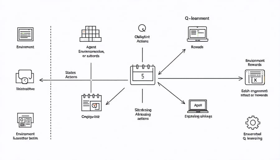
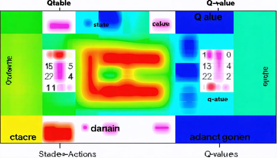
The Q-table is the heart of Q-learning, functioning as a dynamic reference guide that helps your agent make decisions. Think of it as a spreadsheet where rows represent states (where your agent can be) and columns represent possible actions (what your agent can do). Each cell contains a Q-value that indicates the expected reward for taking a specific action in a particular state.
Initially, your Q-table starts with all zeros or random values. As your agent explores and learns, these values are updated based on the rewards received. The reward system is crucial – it’s how you define what constitutes success or failure for your agent. For example, in a maze-solving scenario, you might set up rewards like:
– Positive reward (e.g., +1) for reaching the goal
– Negative reward (e.g., -1) for hitting walls
– Small negative reward (e.g., -0.1) for each move to encourage finding the shortest path
Here’s a simple example of how to create a Q-table in Python:
“`python
import numpy as np
states = 4 # number of possible states
actions = 3 # number of possible actions
q_table = np.zeros((states, actions))
“`
The Q-table updates after each action using the Q-learning formula, which considers both immediate rewards and potential future rewards. This balance between immediate and future rewards is controlled by the discount factor, typically represented as gamma in the code.
Implementing Q-Learning in Python
Creating the Q-Learning Environment
To implement Q-learning in Python, we first need to create a suitable environment that defines our state space and possible actions. Let’s start by setting up a basic grid world environment using NumPy arrays.
First, import the necessary libraries:
“`python
import numpy as np
import random
“`
Create a simple grid environment class that represents your state space:
“`python
class GridWorld:
def __init__(self, size=4):
self.size = size
self.state = 0 # Starting state
self.action_space = [‘up’, ‘down’, ‘left’, ‘right’]
self.n_actions = len(self.action_space)
self.n_states = size * size
“`
Define the core environment functions:
“`python
def reset(self):
self.state = 0
return self.state
def step(self, action):
row = self.state // self.size
col = self.state % self.size
if action == ‘up’: row = max(0, row – 1)
elif action == ‘down’: row = min(self.size – 1, row + 1)
elif action == ‘left’: col = max(0, col – 1)
elif action == ‘right’: col = min(self.size – 1, col + 1)
self.state = row * self.size + col
return self.state
“`
This basic environment provides the foundation for implementing the Q-learning algorithm. The state space is represented as a grid where each cell corresponds to a unique state, and the agent can move in four directions.
Building the Q-Learning Algorithm
Let’s build our Q-learning algorithm step by step in Python. First, we’ll create our Q-table as a dictionary or numpy array to store state-action pairs and their corresponding Q-values:
“`python
import numpy as np
q_table = {} # or use np.zeros((state_space, action_space))
learning_rate = 0.1
discount_factor = 0.95
epsilon = 0.1
“`
The core Q-learning update formula is implemented through this function:
“`python
def update_q_value(state, action, reward, next_state):
current_q = q_table.get((state, action), 0)
next_max_q = max([q_table.get((next_state, a), 0) for a in actions])
new_q = current_q + learning_rate * (
reward + discount_factor * next_max_q – current_q
)
q_table[(state, action)] = new_q
“`
For action selection, we’ll implement the epsilon-greedy strategy:
“`python
def choose_action(state):
if np.random.random() < epsilon:
return np.random.choice(actions) # Explore
else:
return max(actions, key=lambda a: q_table.get((state, a), 0)) # Exploit
```
These components work together in a training loop where the agent interacts with the environment, collects experiences, and updates its Q-values. The agent gradually learns optimal actions for each state by balancing exploration and exploitation through the epsilon parameter.
Remember to adjust the learning rate, discount factor, and epsilon values based on your specific problem requirements. Lower learning rates lead to more stable learning, while higher discount factors emphasize long-term rewards.
Training and Testing the Model
To train your Q-learning model, first initialize the Q-table with zeros and set your hyperparameters like learning rate (typically 0.1-0.4) and discount factor (usually 0.9-0.99). Run multiple episodes where your agent interacts with the environment, updating Q-values using the Q-learning formula after each action.
Monitor the training progress by tracking the total rewards per episode. You should see improvement over time as the agent learns optimal behaviors. A common approach is to use an epsilon-greedy strategy, starting with high exploration (epsilon = 1.0) and gradually decreasing it as training progresses.
To test your model, set epsilon to 0 (pure exploitation) and run several test episodes. Evaluate performance metrics like average reward, completion rate, and steps per episode. Consider saving successful models for use in future AI project implementations.
If results aren’t satisfactory, try adjusting hyperparameters or modifying the reward structure. Remember that finding the right balance between exploration and exploitation is crucial for successful training.
Real-World Application Example
Building a Line-Following Robot
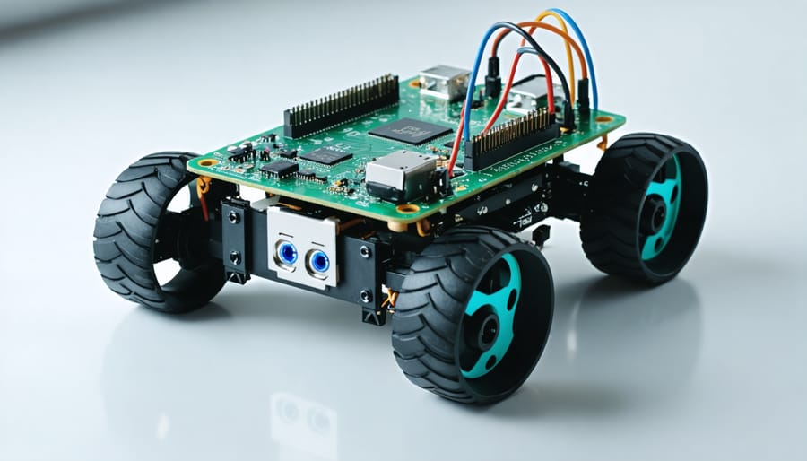
Let’s put our Q-learning knowledge into practice by building a line-following robot. This project combines hardware components with our Python implementation to create a real-world application of reinforcement learning.
For this project, you’ll need a robot chassis, two DC motors, IR line sensors, a Raspberry Pi, and basic electronic components. The robot’s state space consists of readings from three IR sensors (left, center, right), while the action space includes moving forward, turning left, and turning right.
Here’s the core Q-learning implementation for our line-following robot:
“`python
def get_state():
left = GPIO.input(LEFT_SENSOR)
center = GPIO.input(CENTER_SENSOR)
right = GPIO.input(RIGHT_SENSOR)
return (left, center, right)
def take_action(action):
if action == 0: # Forward
set_motors(1, 1)
elif action == 1: # Left
set_motors(0, 1)
else: # Right
set_motors(1, 0)
“`
The reward function assigns positive values when the center sensor detects the line and negative values when the robot strays off course. During training, the robot learns the optimal policy through trial and error, updating the Q-table based on sensor readings and rewards.
We can accelerate learning by implementing a simple exploration strategy:
“`python
epsilon = 0.3
if random.random() < epsilon:
action = random.choice(possible_actions)
else:
action = np.argmax(Q[state])
```
After training for approximately 100 episodes, the robot should consistently follow the line, demonstrating how Q-learning can be applied to solve real-world robotics challenges.
Troubleshooting and Optimization
When implementing Q-learning in Python, you might encounter common issues like slow convergence or unstable learning. To improve performance, consider reducing the learning rate (alpha) if the algorithm is unstable, or increasing it if learning is too slow. Memory usage can become a concern with large state spaces – address this by using sparse matrices or implementing state aggregation techniques.
A key optimization strategy is to implement epsilon decay, gradually reducing random exploration as the agent learns. Start with epsilon at 0.9 and decay it by multiplying with a factor like 0.995 after each episode. This balances exploration and exploitation more effectively.
If your agent isn’t learning effectively, double-check your reward structure. Ensure rewards are properly scaled and meaningful for your specific problem. Additionally, consider normalizing state values to improve learning stability.
For faster execution, vectorize operations using NumPy instead of traditional Python loops. Pre-allocate your Q-table and use efficient data structures. When debugging, implement logging to track the average reward per episode – this helps identify if the agent is actually improving over time.
Q-learning in Python opens up endless possibilities for creating intelligent systems on your Raspberry Pi. By mastering this fundamental reinforcement learning algorithm, you’ve taken a significant step toward building more sophisticated AI applications. Remember to start with simple environments, gradually increase complexity, and thoroughly test your implementations. As you become more confident, explore different reward structures and parameter optimization techniques. For your next steps, consider applying these concepts to advanced machine learning projects or experimenting with variations like Deep Q-learning. The skills you’ve learned here form a solid foundation for more complex reinforcement learning applications. Keep practicing, experimenting, and building – the possibilities are limitless with Q-learning on your Raspberry Pi!